Unleash the Power of Your Report Builder Data: Sorting and Filtering

dotloop

August 07, 2017 | comments

At dotloop, we strongly believe in the power of data — and empowering you with data to run your business as effectively as possible.

Last month, we released the Report Builder, an ad hoc reporting tool allows you to download a CSV file of your loop (transaction) data. Since then, we’ve received some questions about how to slice, dice, and analyze the data in your CSVs, and wanted to offer some guidance on how to do your own analysis.

Below, you’ll learn how to use Excel to sort and filter your data.

How to Sort/Filter Data

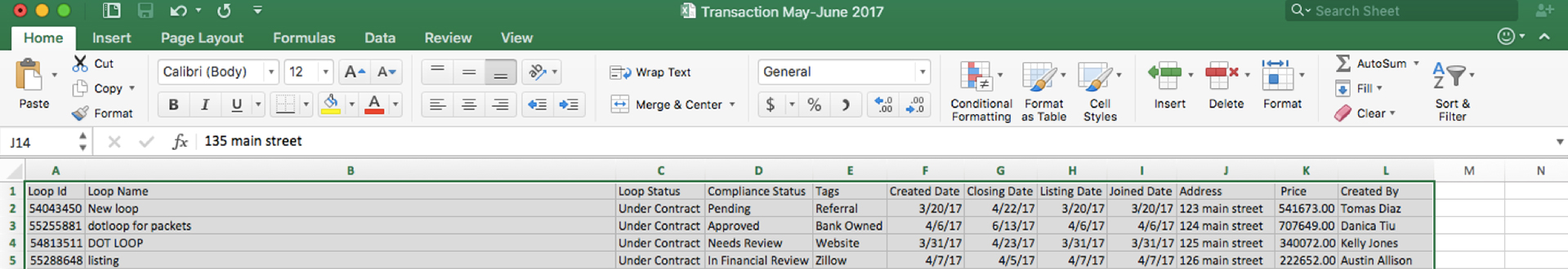
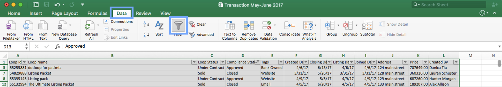
STEP 1: Select all data/columns in the CSV file

Make sure to select all columns! If you don’t, you’ll run into some sorting and filtering problems – namely, the selected columns will be sorted and filtered, while the unselected columns will remain unchanged.

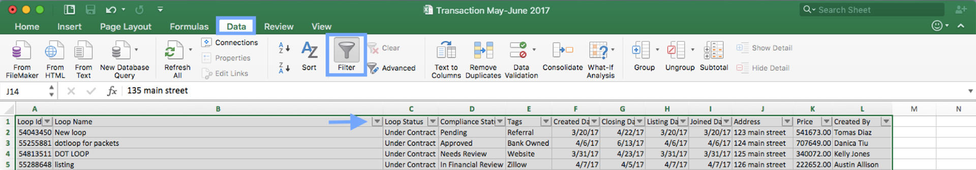
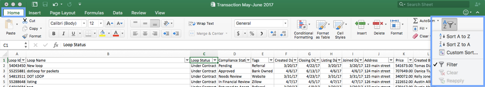
STEP 2: Select the DATA tab, then click on the FILTER button.

A drop-down arrow will appear next to each column header. When you click this arrow, you will see options to filter or sort your data. Play around with this feature: you can sort from largest to smallest, smallest to largest, etc.

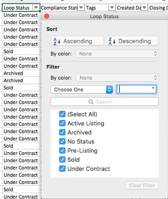
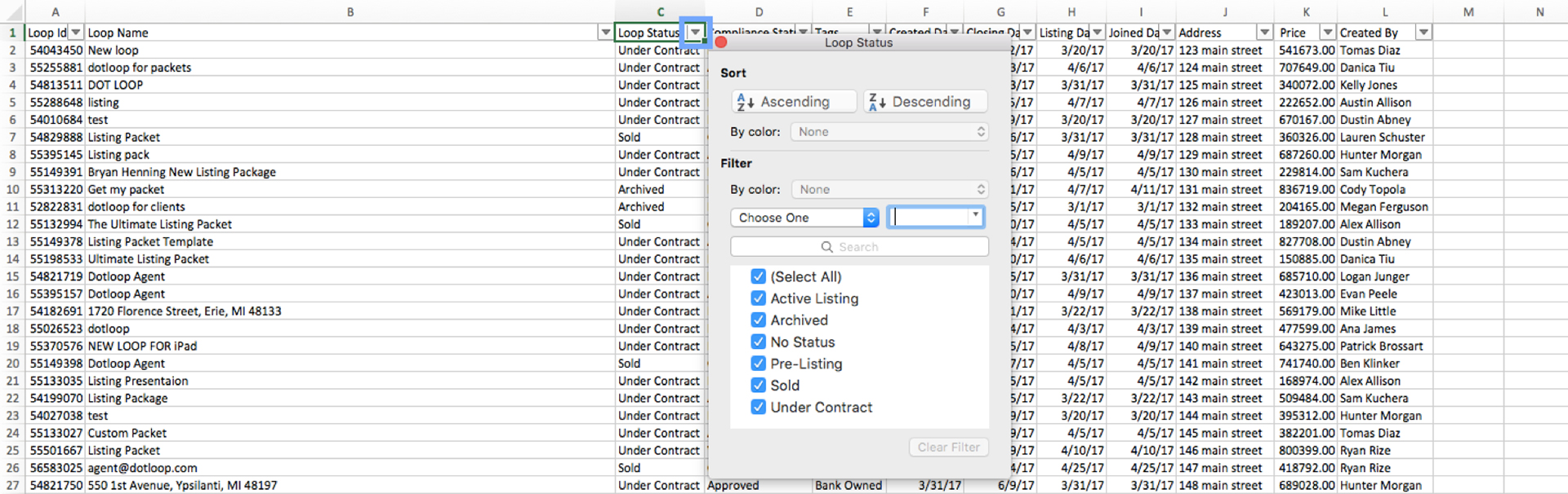
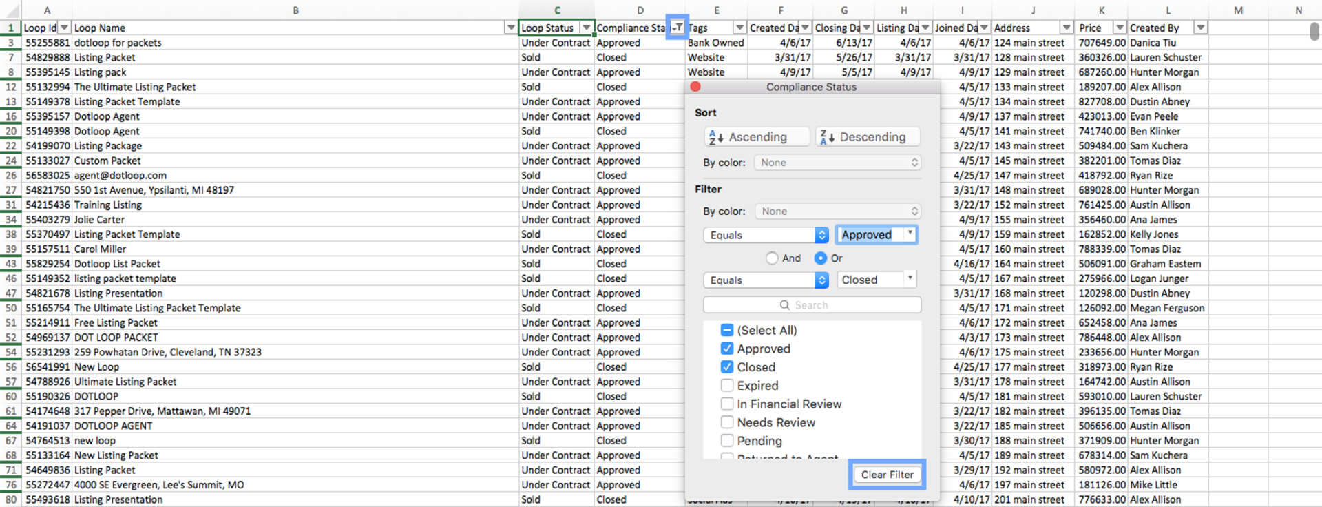
STEP 3: Customize your filters

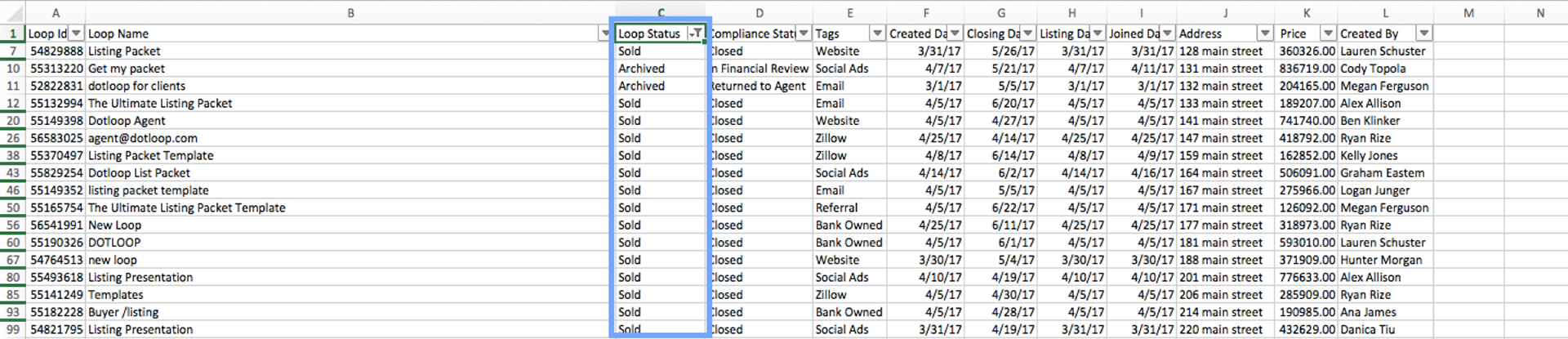
If you would like to apply a filter to your data, click on the drop-down arrow next to the header of the column you would like to filter, and the filter menu will appear. To easily deselect all of the column options, un-check the SELECT ALL box. To select one of the options — or multiple, depending on what you’re filtering for — then hit OK. The checked options will be the only ones that show up on the spreadsheet; note that your other cells have not been deleted, but have just been temporarily hidden.

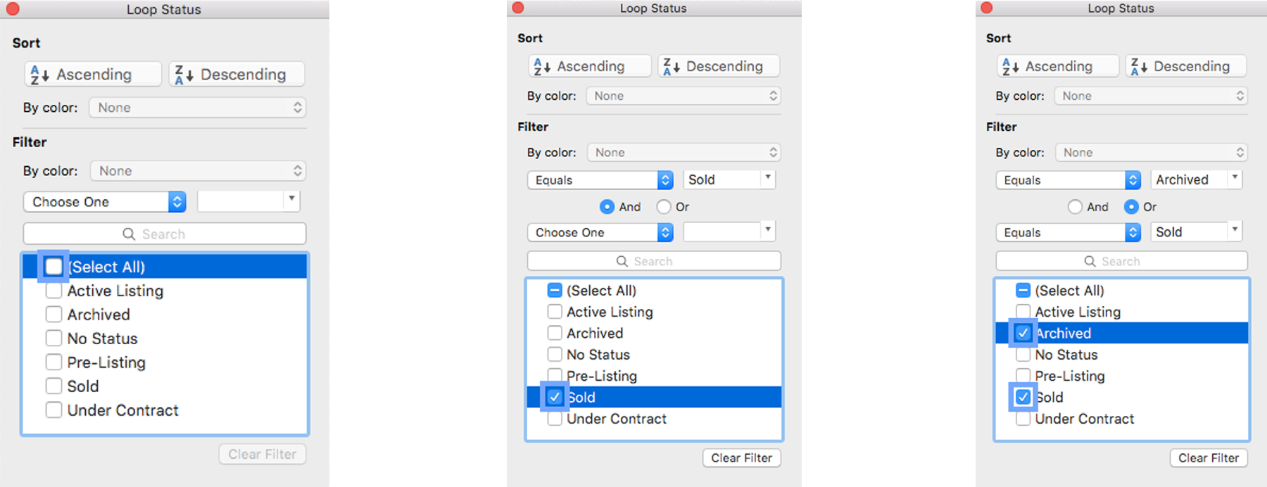
** Alternatively, you can use the Sort/Filter button on the HOME tab at the top of the Excel spreadsheet to filter.

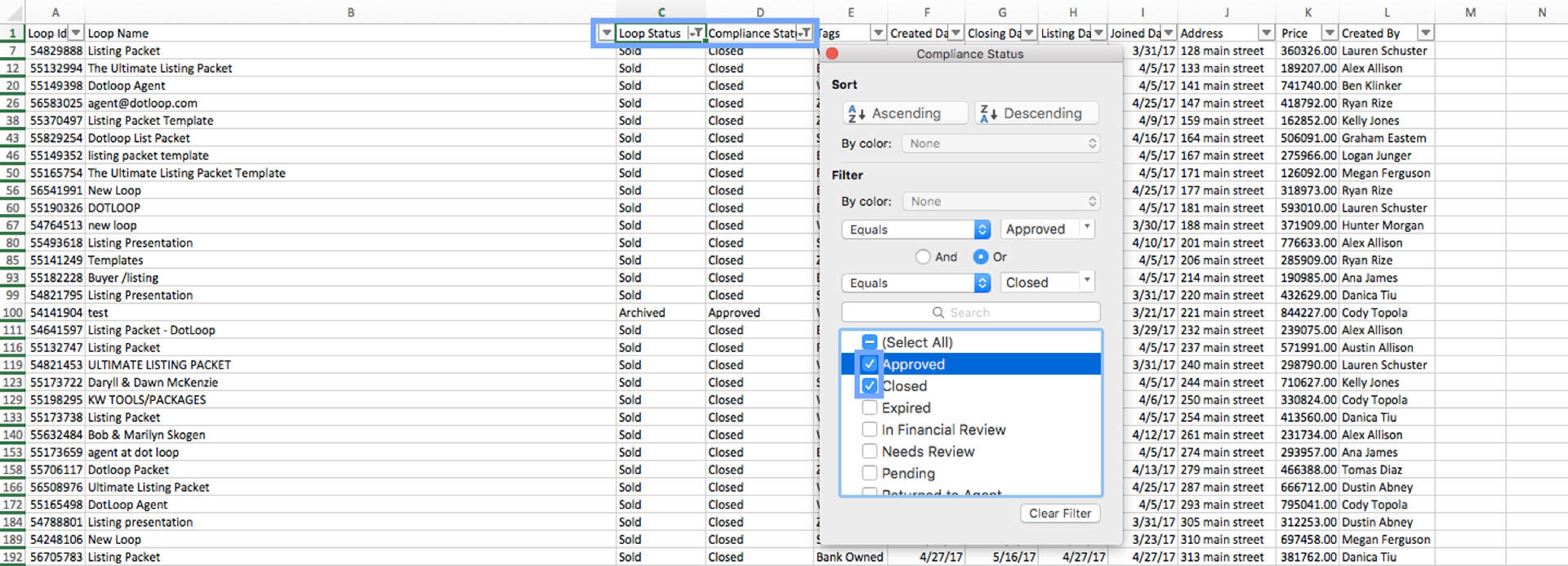
How to Apply Multiple Filters to Your Data

To further narrow down your data, you can apply multiple filters to your data. To do so, select the drop-down option next to the second column you would like to filter by. Then, uncheck all of the options that you would like to remove from the spreadsheet, or uncheck SELECT ALL and check only the options you would like to remain. The spreadsheet will now only show data that matches the criteria for the filters that have been applied.

To continue narrowing down your data, you can continue applying filters on as many columns as you would like.

How to Clear Filters

To clear or remove one, multiple, or all filters, click on the drop-down arrow for the filter you would like to clear/remove and select the CLEAR FILTER FROM “[Column Name]”. This will remove the filter and the data that was being temporarily hidden by the filter will be unhidden.

** For a quick way to remove all filters from the data, deselect the FILTER button on the DATA tab.

If you would like to learn more about the Report Builder check out our recorded webinar.